BARCODE 2.0 Tutorial
1 | Installation
The BARCODE source code can be directly downloaded on any system running Python 3.12 or later from the BARCODE-HTP Github repository.
BARCODE requires the following packages which are listed in the source code file requirements.txt:
ImageIO: Version ≥ 2.34.1
Matplotlib: Version ≥ 3.8.4
ND2: Version ≥ 0.10.1
Numpy: Version ≥ 2.0.1
OpenCV: Version ≥ 4.10.0.84
PIMS: Version ≥ 0.6.1
PyYAML: Version ≥ 6.0.2
Scipy: Version ≥ 1.14.0
Scikit-Image: Version ≥ 0.24.0
BARCODE was developed on the package versions listed above, and may not work on previous versions of the listed software packages.
To install the required packages run the command: pip install -r requirements.txt
To run BARCODE, navigate to the source code directory in the terminal and run the command: python main.py or python3 main.py
This tutorial walks users through how to run BARCODE and interpret outputs. Further details about BARCODE algorithms and output metrics are described in the BARCODE Metrics page and ReadMe.
3 | General Walk-through
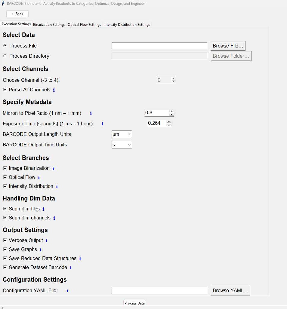
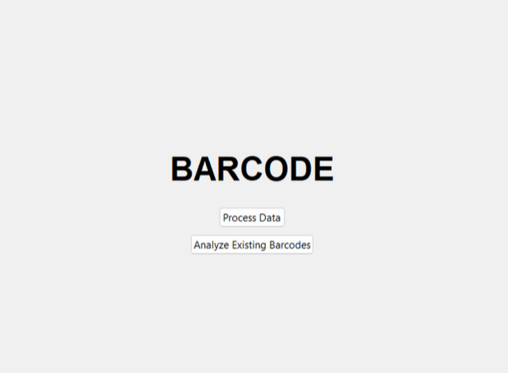
The opening screen contains two main options:
Process Data and Analyze Existing Barcodes.
The Process Data option is used to run BARCODE analysis on new microscopy files or folders. This tutorial focuses on this feature which has all of the primary BARCODE algorithms described in Section 4.
The Analyze Existing Barcodes option is used for post-processing previously generated BARCODE CSV files and reduced data structures. Details are provided in Section 5.
Execution Settings
In the Execution Settings tab, use Process File to choose a single file, or use Process Directory to choose an entire folder. The Browse File button allows the user to search the file system for acceptable microscopy files, while the Browse Folder button allows the user to select a directory for batch processing. Then, choose whether BARCODE should analyze a specific channel or all channels in the selected data. The Choose Channel setting is used to select a single channel, while Parse All Channels scans every available channel in each video. Selecting a channel less than 0 will result in reverse indexing of channels. For example, selecting −1 will run the program on the last channel of every video scanned, rather than the first. When first using the BARCODE application, it is recommended to start with a single channel of a single file. This allows the user to test the selected parameters and verify that the output is reasonable before processing an entire dataset.
The Execution Settings tab also includes metadata and unit settings. The Micron to Pixel Ratio and Exposure Time settings are used for converting optical flow outputs into physical units. Note that for most applications the exposure time is the frame interval. For .nd2 files, these values may be read automatically from the file metadata. The Length Unit and Time Unit settings control the physical units used in output labels and unit conversions.
In the general execution settings, it is recommended that the user turn on the three main analysis branches: Image Binarization, Optical Flow, and Intensity Distribution. These selections control which branches of the program are run on the data. When all three branches are enabled, BARCODE 2.0 provides 25 analysis metrics: 12 from the Image Binarization branch, 6 from the Intensity Distribution branch, and 7 from the Optical Flow branch. Disabling one or more branches may result in faster runtime, but fewer metrics will be calculated for each video.
The ‘dim’ data settings allow the user to choose whether BARCODE should process files or channels that have low contrast, which we classify as ‘dim’ using the criterion that the minimum intensity is greater than or equal to 2/e times the mean intensity in the first frame. The Scan dim files option allows dim files to be processed, and the Scan dim channels option allows dim channels to be processed. Turning these settings on will enable the program to process these videos. In the summary CSV output, the Flag column will return 1 if the video or channel is dim (Flag = 0 if it is not dim).
The Verbose Output setting provides additional information while the data are being processed, including progress updates, processing time, and whether an input video was classified as dim.
The Output Settings control files generated by BARCODE in addition to the summary CSV file. The Save Graphs setting saves PNG visualizations of selected analysis outputs. The Save Reduced Data Structures setting saves the reduced data structures, such as binarized images, optical flow fields, and intensity distributions, as CSV files for offline analysis or verification. The Generate Dataset Barcode setting creates a color-coded BARCODE image file for the dataset. This barcode provides a compact visual summary of the output metrics for the analyzed files and channels.
Post-processing
After the application is run on a file or directory, BARCODE creates output files in the selected data location. These outputs include the summary CSV file and, depending on the selected settings, visualizations, reduced data structures, a graphical barcode png, run time information, and a YAML configuration file that stores the selected settings from the run. This file can be loaded later using the Configuration YAML File option, allowing the same settings to be reused for future datasets.
For previously generated BARCODE outputs, users can return to the home screen and select Analyze Existing Barcodes. This page contains tools for combining CSV files, generating aggregate or comparison barcodes, comparing two selected metrics, and visualizing saved reduced data structures. These post-processing tools are described in later sections of this tutorial.
4 | Adjusting Parameters
This section discusses how changing parameters affects the output BARCODE and why you may or may not want to adjust these parameters.
4.1 | Downsampling and Averaging
Frame Step
To increase processing speed and reduce the data size, videos can be downsampled in time by choosing to analyze every kth frame. This Frame Step parameter (k) allows the customization of the speed and precision of each branch. We have found that k = 10 typically provides sufficient resolution and accuracy for all branches while maintaining rapid processing times. Frame Step is set separately for the Image Binarization, Optical Flow, and Intensity Distribution branches. Increasing the frame step decreases runtime, but may reduce temporal resolution in the corresponding branch.
Percentage of Frames for analyzing changes in metrics
The frame start and end percentage sets the percentage of frames X at the beginning and end of the video used to compute the change in the various metrics such as maximum island area change, maximum void area change, speed change, kurtosis change, median skewness change, and mode skewness change. By default, these metrics compare the change in values averaged over the first 5% and last 5% of frames in the video. Increasing X can reduce noise by increasing the number of frames that contribute to the quantity, but will also reduce temporal resolution.
4.2 | Binarization Settings
Binarization Threshold
The Binarization Threshold determines what pixels within the image represent material or mass, which we assign the value of 1, and which are background or noise, which we assign a value of 0. The Binarization Threshold is calculated for each frame as
((1 + Offset) * Mean Pixel Intensity).
Users should take care when adjusting this value, as it can affect the results of the Binarization Branch. As the threshold decreases, more noise may be included. As the threshold increases, material features may be lost.
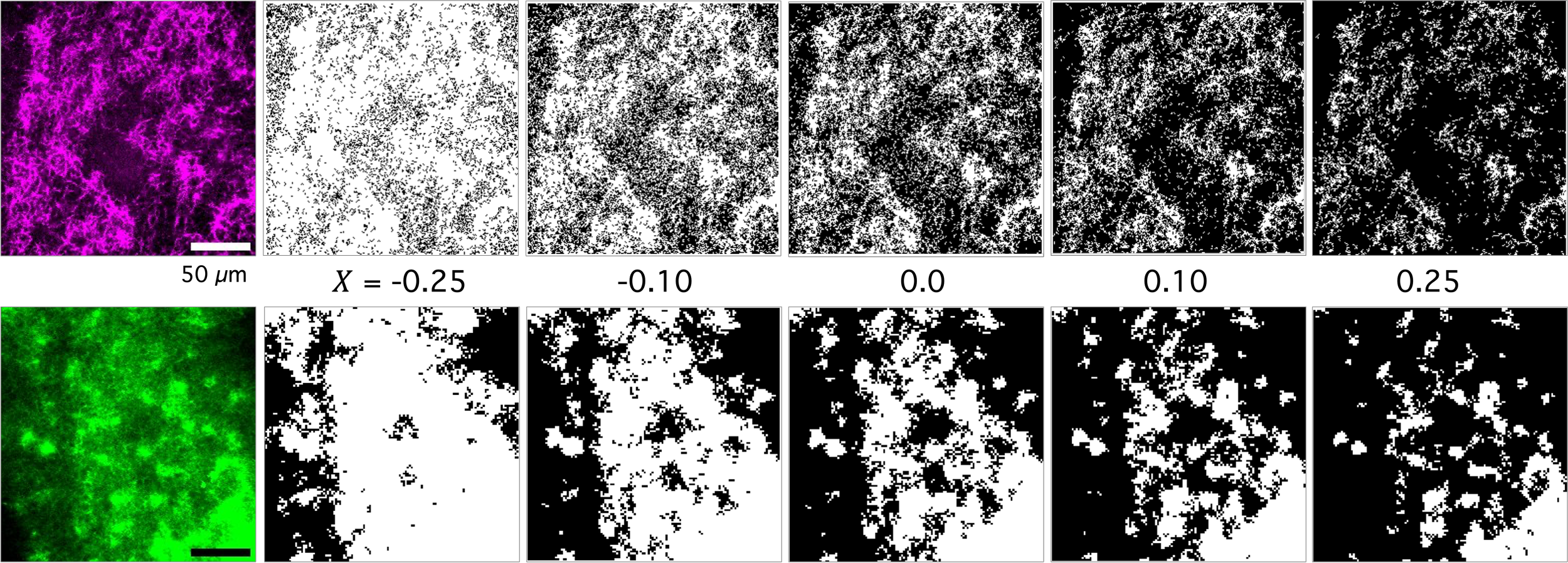
4.3 | Intensity Distribution Settings
Number of Bins
The Intensity Distribution branch calculates the mode skewness, median skewness and kurtosis by binning the pixel intensity values for the selected frames, and then calculating the metrics on these distributions. The default number of bins is set to 300. Adjusting this parameter will adjust the number/width of the bins used to create the distribution. Increasing the number of bins may more precisely capture pixel intensity values, but may result in noisier data, while decreasing the number of bins will result in less precision in the estimation of pixel intensity counts.
Noise Threshold
The distribution noise threshold determines the minimum pixel intensity probability allowed within a single bin for that bin to be evaluated. All bins with a normalized probability below this threshold will be removed from the calculation, and the distribution renormalized to ensure that the integrated probability = 1. The default noise threshold is set to 0.0005. Decreasing this value can result in noisier data and potential inaccuracies in the calculation of the kurtosis and skewness metrics, while increasing this value can result in fewer pixels being counted towards the Intensity Distribution branch metrics.
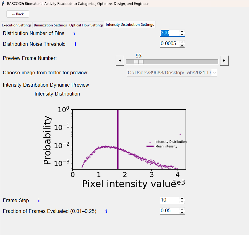
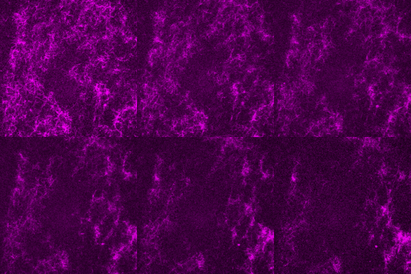
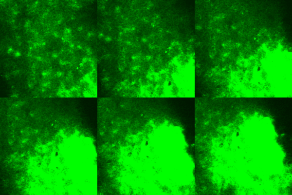
(Left) First frame of Video 1 (top, magenta) and Video 2 (bottom, green). (Right) Binarized images with different threshold values X applied to the image. The best offset value in these examples are between 0.1 and 0.25. Default value in BARCODE is set to X=0.1 (X=10%).
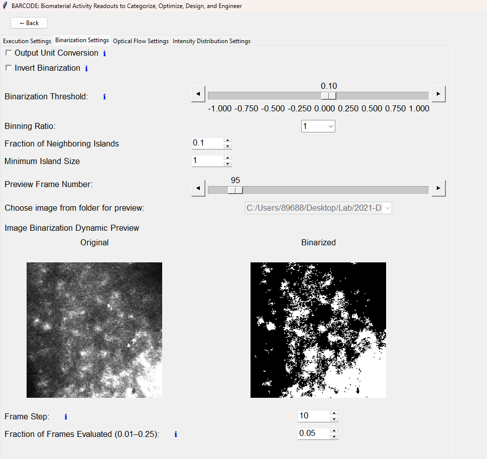
The Binarization Settings tab includes an Image Binarization Dynamic Preview (shown to the left).
This preview shows the original image and the binarized image side by side, allowing users to adjust the threshold and inspect the effect before running the full dataset.
Binning Ratio
The Binning Ratio controls the extent of spatial downsampling performed before binarization. The image is averaged over p x p pixel regions, reducing noise and decreasing data size. Larger binning ratios can improve processing speed and reduce noise, but may also remove small spatial features. The default binning ratio is 2.
Output Unit Conversion
The Output Unit Conversion setting changes selected image binarization area metrics from field-of-view percentage units to physical area units based on the selected length unit. This uses the micron-to-pixel ratio from the Execution Settings or the metadata read from .nd2 files.
Invert Binarization
The Invert Binarization option reverses the binarized image. This can be useful when the material and background intensities are inverted relative to the default assumption that the material is white (1) and background is black (0).
Fraction of Neighboring Islands
The Fraction of Neighboring Islands parameter is used to calculate Mean Island Separation. After binarization, BARCODE identifies each island and calculates the centroid of each island. For each island, the program then measures distances to nearby island centroids. This parameter controls how many neighboring islands are included in that distance calculation.
For example, if this default value is set to 0.10, BARCODE uses approximately the closest 10% of islands when estimating the local island separation. Smaller values emphasize local spacing between nearby islands, while larger values include more distant islands and produce a more global estimate of island separation.
Minimum Island Size
The Minimum Island Size parameter can be used to reduce the influence of very small islands that may represent noise. Increasing this value filters out smaller connected components during binarization-based analysis and preview.
The Intensity Distribution Settings tab includes an Intensity Distribution Dynamic Preview (shown to the left).
This preview shows the distribution for a chosen frame allowing users to adjust the settings and inspect the effect before running the full dataset.
4.4 | Optical Flow Settings
Window Size
The Optical Flow Window Size parameter defines the size of the region around each pixel that is used to compute the local motion within the optical flow algorithm. Larger window sizes result in less noise being captured by the algorithm, but will result in less resolved motion fields, while smaller window sizes are more capable of detecting smaller movement within the material, but will be more susceptible to random noise.
Downsampling
Depending on the scale of movement within the data, it is possible to spatially downsample the image array by a Downsample/Binning Factor (p), which can drastically increase the throughput of the Optical Flow measurements. The extent of downsampling is set by averaging together p×p regions of pixels, which reduces the original m×n field of view to a downsampled array of m/p×n/p pixels. Increasing p suppresses noise and improves detection of bulk movement while also reducing spatial resolution. It also increases processing speed and reduces the RDS size. We have found p= 2-8 to provide sufficient resolution and accuracy while maintaining rapid processing times. The default value is set to p=8.
Note: Care should be taken in downsampling videos that capture the movement of many smaller areas of material, as these small scale motions may be lost in the averaging.

(Left) First frame of Video 1 (top, magenta) and Video 2 (bottom, green). (Right) Flow fields generated from the Optical Flow Branch with different downsampling values p. Default value in BARCODE is set to p=8
Calibration parameters
The micron-to-pixel ratio and exposure time are determined by the image acquisition settings. Allowable values of micron-to-pixel ratio range from 0.001 to 1000 microns per pixel. Allowable values of exposure time range from 0.001 to 3600 seconds. For .nd2 files, these parameters are automatically read using the file metadata.
The Micron to Pixel Ratio and Exposure Time settings are located in the Execution Settings tab under Specify Metadata. The Length Unit and Time Unit settings control output labels and physical unit conversions.
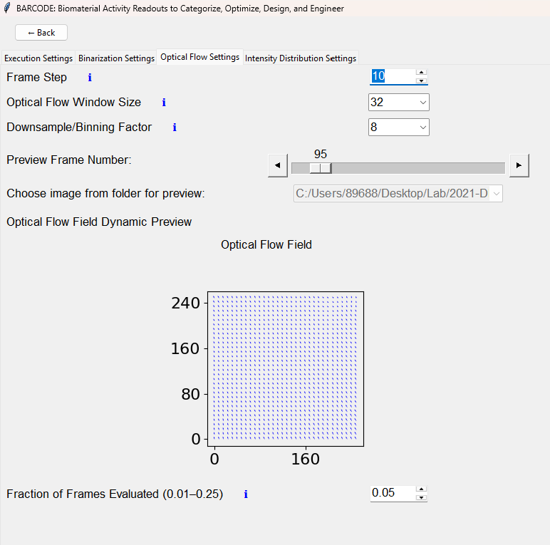
The Optical Flow Settings tab includes an Optical Flow Field Dynamic Preview (shown to the left).
This preview shows the flow field for a chosen frame allowing users to adjust the settings and inspect the effect before running the full dataset.
5 | Analyzing Existing Barcodes
BARCODE 2.0 includes a workflow for analyzing previously generated BARCODE summary CSV files and reduced data structures by selecting Analyze Existing Barcodes from the home screen.
This workflow is especially useful for larger studies where image analysis has already been completed. Users can revisit the output files, generate aggregate summaries, compare datasets using consistent color limits, or export selected metric comparisons for further statistical analysis.
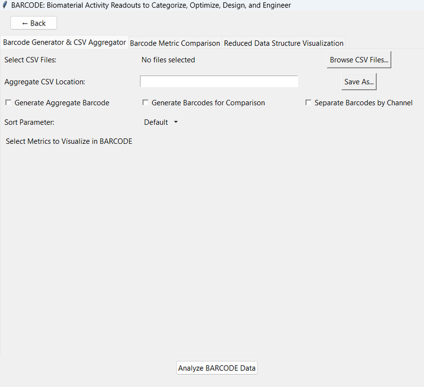
Barcode Generator & CSV Aggregator
The Barcode Generator & CSV Aggregator tab allows users to select one or more BARCODE summary CSV files and combine them into a single aggregate CSV file. This is useful when results from multiple files, folders, experimental conditions, or replicates need to be assembled into one dataset. Users can choose whether barcodes should be separated by channel, choose an output location for the aggregate CSV file, and generate an aggregate barcode visualization. The aggregate barcode provides a compact color-coded representation of the selected metrics across all included samples.
When Generate Barcodes for Comparison is selected, BARCODE creates barcode visualizations for each input CSV using consistent metric limits, which makes it easier to visually compare datasets because the same colors correspond to the same metric ranges across all generated barcodes.
A Sort Parameter can be selected to organize the data from least to greatest along a chosen metric. If the sort parameter is left as Default, the files will be organized in the order of selection and by alphabetical order within the selected folder(s).
The Select Metrics to Visualize in BARCODE option allows users to choose which metrics are included in the barcode visualization, when a user wants to focus on a subset of metrics rather than displaying all available metrics
Reduced Data Structure Visualization
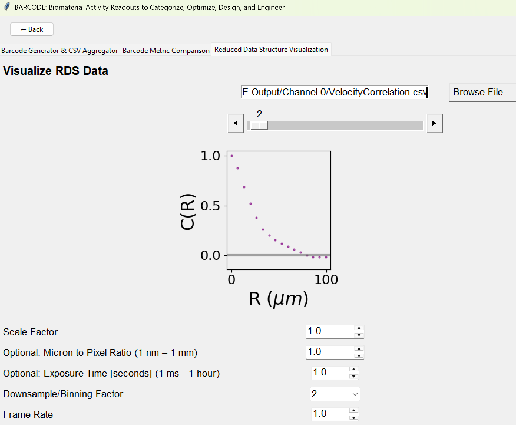
The Reduced Data Structure Visualization tab allows users to inspect saved reduced data structure files generated by BARCODE. These files may include binarized images, optical flow fields, intensity distributions, spatial autocorrelation data, velocity correlation data, and related intermediate outputs.
After selecting a reduced data structure CSV file, users can move through frames using the preview frame slider. Depending on the selected RDS type, BARCODE displays the corresponding image, vector field, intensity distribution, or correlation distribution.
This allows users to visually inspect intermediate outputs and verify that the analysis results are reasonable. This tool is also useful for quality control and troubleshooting. For example, users can check whether binarization accurately captures material structures, whether optical flow vectors are reasonable, or whether correlation functions behave as expected.
The preview can also be saved as a single frame or as a video using the right-click menu. For correlation data, users can also save all correlation distributions together for easier comparison across frames.
6 | Reading Barcodes
After generating the barcode for a dataset, how should it be interpreted? The barcode matrices provide a compact way to compare the output metrics across videos, channels, and datasets. In a barcode visualization, each row corresponds to an analyzed file or file-channel entry, and each column corresponds to one BARCODE metric. The color in each cell represents the normalized value of that metric for that entry.
The full BARCODE 2.0 output contains 25 analysis metrics: 12 metrics from the Image Binarization branch, 6 metrics from the Intensity Distribution branch, and 7 metrics from the Optical Flow branch. These metrics describe material connectivity, island and void areas, island morphology and separation, structural correlation, intensity distribution shape, flow speed and direction, velocity correlation, divergence, and curl. A detailed mathematical description of all 25 BARCODE metrics is described in the BARCODE Metrics page.
The barcode is intended to give a quick visual summary of the dataset. Samples with similar color patterns across the metric columns have similar BARCODE profiles, while samples with different color patterns may represent different material structures or dynamics.
The “plasma” color scale is applied separately to each metric. This means that colors should be interpreted column by column, rather than as absolute values across different columns. For example, a bright color in one metric column indicates a relatively high value for that metric, but it should not be directly compared to the same color in a different metric column unless the color scales are considered. The exact values for each metric can be found in the summary.csv file.
For a standard aggregate barcode, the color limits are calculated from the data included in generating that barcode. Therefore, colors are best interpreted within the same barcode visualization. For direct comparison across multiple datasets, the Generate Barcodes for Comparison option generates barcodes for multiple CSV files using consistent metric limits. This allows the same colors to represent the same metric ranges across the comparison barcodes.
Barcode Metric Comparison
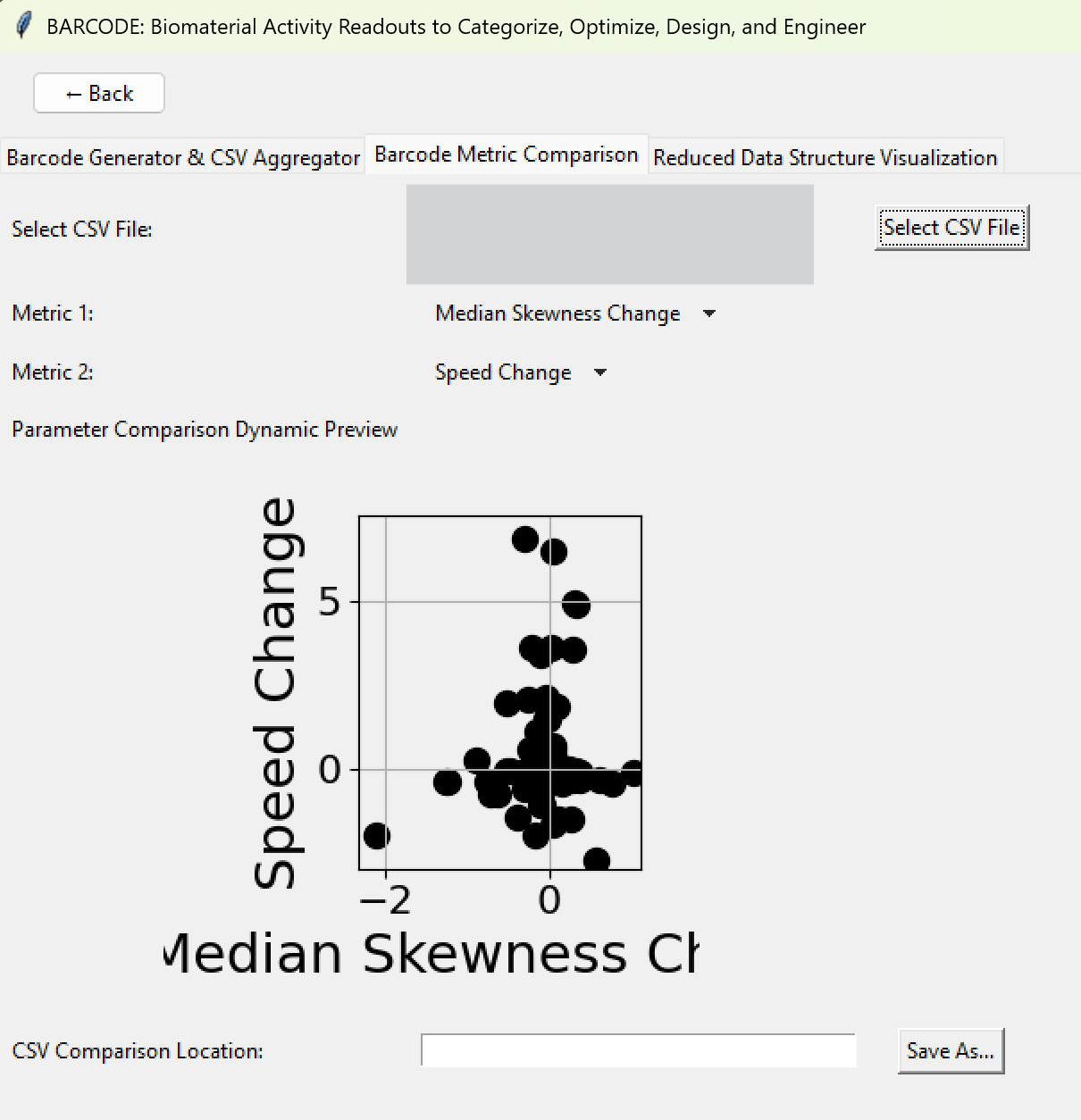
The Barcode Metric Comparison tab allows users to compare two selected BARCODE metrics from a summary CSV file.
After selecting a CSV file, users choose Metric 1 and Metric 2. BARCODE then generates a dynamic preview plot showing the relationship between the two selected metrics across the samples in the CSV.
This feature is useful for quickly checking relationships between BARCODE outputs. The selected metric pair can also be exported as a new CSV file for further plotting or statistical analysis.
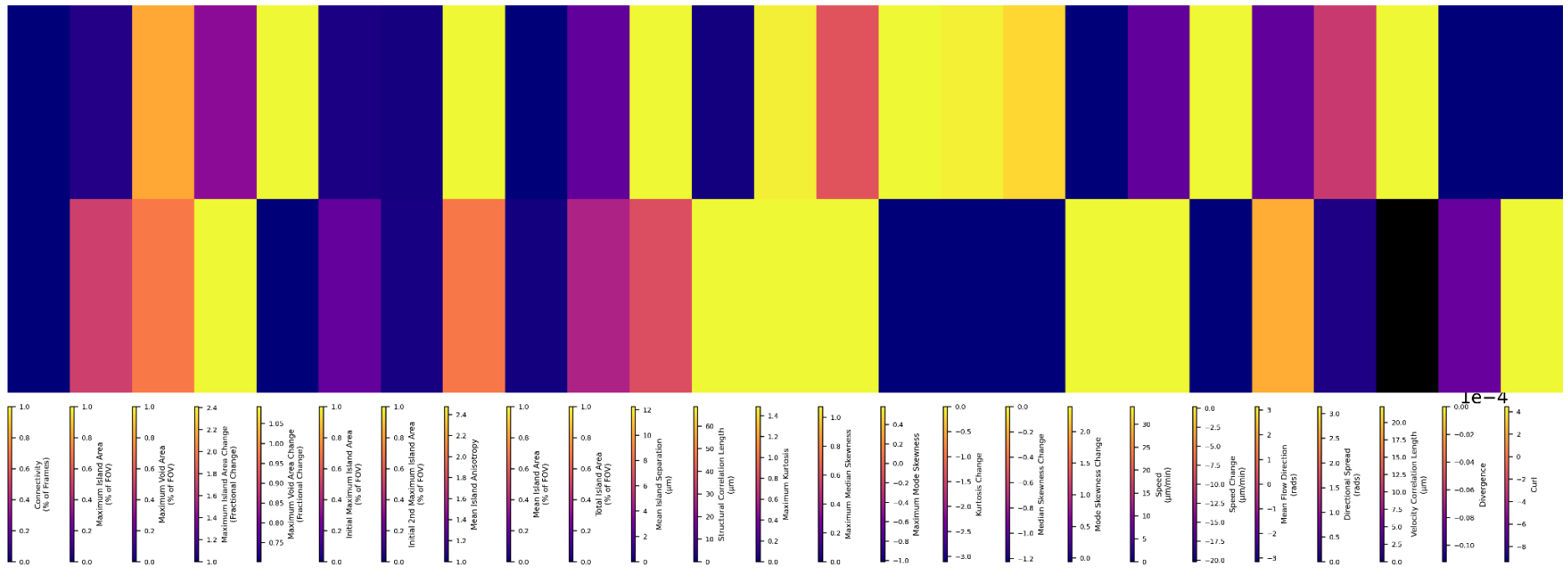
Users can also select which metrics are shown in the barcode visualization. If the Select Metrics to Visualize in BARCODE option is used, the barcode may display only a subset of the full 25 analysis metrics. This can be helpful when focusing on a smaller group of metrics for a specific comparison.
If Separate Barcodes by Channel is selected, BARCODE generates separate barcode visualizations for each channel. This can make it easier to compare samples within the same channel and avoid mixing results from different imaging channels in one visualization.
When interpreting barcodes, users should also consider whether all analysis branches were run. If a branch was not selected during processing, the metrics from that branch will be saved as NaN values in the summary CSV file and may appear as missing or black cells in the barcode visualization.
BARCODE 2.0 summary files also include a flag column that indicates potential issues with the reliability of some outputs. These flags should be checked when interpreting the barcode and summary CSV output.
Flag = 0: no warning was detected.
Flag = 1: dim file or channel - defined as videos where the first frame has a minimum pixel intensity greater than or equal to 2/e times the mean pixel intensity of the corresponding frame.
Flag = 2: saturated file or channel - if the mode of the pixel intensity distribution coincides with the maximum intensity bin of the histogram in every analyzed frame. If even one analyzed frame does not satisfy this condition, no saturation warning is reported.
Flag = 3: structural image autocorrelation (SIA) correlation length exceeds the field of view in at least one analyzed frame.
Flag = 4: velocity correlation length exceeds the field of view in at least one analyzed frame.
Barcodes are most useful for identifying broad trends, comparing samples, and selecting datasets or conditions for closer inspection. For more detailed interpretation, users should examine the corresponding summary CSV file, saved visualizations, and reduced data structures.
7 | FAQs
-
No, files must be converted to .tif or .nd2 to analyze with the BARCODE application. Follow Section 2 to convert your files to the correct format.
-
Yes, the program has no issue when executing folders with multiple acceptable file types.
-
The easiest way to speed up the BARCODE execution is to increase the Frame Step or decrease the Percentage of Frames.
-
We recommend using BARCODE 2.0, which has the most up-to-date features and functionality. Prior releases are still available, if you prefer to use a legacy version of the software for continuity. All BARCODE releases and associated content can be found here.
-
Yes, BARCODE is open-source software available under a BSD 3-Clause License. Copyright (c) 2025, The Regents of the University of California. Full details can be found here.
-
Please cite this publication, which describes the development and core features of BARCODE:
Chen Q, Sriram A, Das A, Matic K, Hendija M, Tonry K, Ross JL, Das M, McGorty RJ, Robertson-Anderson RM, Valentine MT. BARCODE: high throughput screening and analysis of soft active materials. Nature Communications. 2025. https://doi.org/10.1038/s41467-025-67963-3
To analyze a new file, select Process Data.
The screen to the left is what the user-interface looks like once you click ‘Process Data’.
It shows the Execution Settings interface which is described below.
There are also 3 branch-specific tabs which will be described in Sections 4.2-4.4:
Binarization Settings
Optical Flow Settings
Intensity Distribution Settings
These tabs include branch-specific settings and dynamic previews that can be used to evaluate and adjust branch-specific settings before running the full analysis. The previews can also be saved as a single frame or as a video using the right-click menu.